Scheduling Algorithms: Linux O(1)

Nearly fifteen years ago, just as I was starting my career, Linux released its landmark 2.6 kernel. In this release that everyone had been eagerly anticipating, the most exciting feature was the O(1) scheduler. This article discusses how the algorithm is implemented. Before explaining the O(1) scheduler in detail, however, let us briefly revisit the long-criticized 2.4 scheduler—to understand its lineage and, as the saying goes, use history as a mirror.

The Problems with the 2.4 Scheduler

The Linux 2.4 scheduler supported SMP (Symmetric Multi-Processing). However, because it used a single global runqueue, every core had to compete for tasks in the same runqueue, which hurt scalability. I mentioned this in my previous article:

How should tasks be organized? Should all resources share a single task runqueue, with the scheduler using locks during scheduling to guarantee mutual exclusion, or should we give each resource its own runqueue to reduce lock overhead? That raises another question: if the task list on a given resource becomes empty, should the resource sit idle, or should it go to another resource’s runqueue and “steal” tasks to execute?

The 2.6 O(1) scheduler solved this with per-core runqueues; we will set that aside for now.

The performance cost of the global runqueue was actually still tolerable—after all, locks were needed only during dequeue. The next problem, however, was deadly: the 2.4 scheduler had O(N) time complexity. Modern operating systems can run thousands upon thousands of processes, and an O(N) algorithm means that at every scheduling decision, for the process that has just finished executing, the scheduler must scan all processes in the expired queue to find the right position at which to insert it. This not only causes a huge loss in performance but also makes scheduling latency highly variable—depending on system load, it could differ by several times or even hundreds of times. As we know, nondeterminism is a mortal enemy of software systems, especially real-time systems.

For those less familiar with the 2.4 scheduler, a few more words: it maintained two queues—the runqueue and the expired queue. Both queues were always kept sorted. When a process exhausted its time slice, it was inserted into the expired queue. When the runqueue became empty, one simply swapped the runqueue and the expired queue.

Note that the hard part of any scheduling system is not finding the next runnable process; that operation is usually O(1), since we need only keep the runqueue properly ordered so that its first process is always the one to be scheduled next. The hard part is the process that has finished executing—how do we insert it in the right place so that the runqueue remains sorted?

What Data Structures Can Possibly Satisfy an O(1) Scheduler?

From what we learned in data structures courses, for most algorithms O(log N) is essentially the best achievable result. So how did the 2.6 O(1) scheduler do it?

Before answering that question, let us review the four basic operations on data structures and their time complexities:

• access: random access. An array is the only data structure that can achieve O(1) random access in both the average and worst cases. For other structures, a linked list is O(N), and a tree is generally O(log N).
• search: searching. When it comes to search, everyone’s first reaction is that a hash table has O(1) time complexity. However, in the worst case it is O(N). Apart from that, no algorithm can search in O(1) in the worst case. Most trees (B-trees / red-black trees) are O(log N) in both the average and worst cases, making them the next best option.
• insert/deletion: insertion and deletion. Insertion and deletion are symmetric operations, so we discuss them together. Linked lists, stacks, and queues are O(1) in both the average and worst cases. The hash table in everyone’s mind, likewise, is O(1) on average but O(N) in the worst case. Most trees (B-trees / red-black trees) are O(log N) in both the average and worst cases, which is not bad either.

So we can see that to achieve an O(1) scheduler, the operations can include only pure access, insert, and deletion. There absolutely must be no search. The 2.4 scheduler used search when inserting a finished process back into the expired queue, greatly degrading the overall time complexity of the algorithm. That is point one.

In addition, when choosing an algorithm for a scheduler, we should try to choose one whose average-case and worst-case behavior are consistent. If the average case is O(1) but the worst case is O(n), the scheduler will introduce great nondeterminism into the system, which is a real headache—after all, no one wants to deal with a system that behaves beautifully most of the time but goes utterly haywire in extreme cases. That is point two.

Given these two preconditions, our range of choices becomes narrow—random access can only use an array, and insert/delete can only use a linked list/queue/stack.

Next, let us simplify the scheduling scenario: suppose there are six processes in the system and three priority levels—high, medium, and low. There is no preemption, and processes execute strictly in priority order. How, then, do we combine the data structures above so that scheduling is O(1)?

Think about it.

Think again.

2.6 O(1) Scheduler

OK, let us look directly at the answer the masters came up with. First, the diagram:

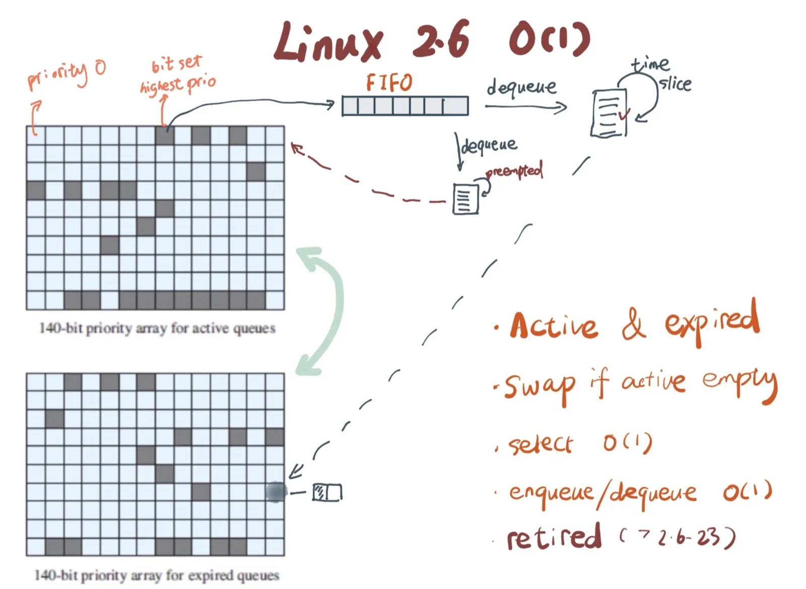
At this point, some readers have probably already grasped the essence. The 2.6 kernel has 140 priority levels, so we use an array of length 140 to record priorities. Under each priority, a FIFO queue manages the processes at that priority. New arrivals go to the tail of the queue; first in, first out. In this case, both insert and deletion are O(1).

So how do we find the runnable process at the current highest priority? If we iterate from 0 all the way down, the algorithm is not O(N) but O(M), where M is the number of priority levels; nor can it be considered O(1). In the 2.6 scheduler, the clever designers of old adopted a bitarray. It allocates one bit per priority level: if the priority queue contains any processes, the corresponding bit is colored—set to 1—otherwise it is set to 0. The problem is thus reduced to finding the highest set bit (the left-most bit) in a bitarray, which is essentially a single CPU instruction (fls).

Good—the general idea is now complete. Let us walk through the full set of steps:

1. In the active bitarray, find the position x of the left-most bit.
2. In the active priority array (APA), locate the corresponding queue, APA[x].
3. Dequeue a process from APA[x].
4. For the process that has just finished executing, recalculate its priority, then enqueue it into the corresponding queue EPA[priority] in the expired priority array (EPA).
5. If the corresponding bit for that priority in the expired bitarray is 0, set it to 1.
6. If the active bitarray is all zeros, swap the active and expired bitarrays.

Of course, there are some details here. For example, if a process is preempted and has not used up its time slice, then in step 4 it is enqueued back into the active priority queue. But this has little to do with the algorithm itself, so we will skip it.

Its Place in History

The 2.6 O(1) scheduler has now been replaced by CFS (the Completely Fair Scheduler), which is slightly inferior in raw performance but places greater emphasis on fairness. Yet with its distinctive design and simple algorithm, it influenced many systems. When it first appeared, many Linux distributions could not wait to port it back to the 2.4 kernel. And in several schedulers I have encountered throughout my career as a programmer, the imprint of bitarray + priority queue can be seen. It makes me marvel at the beauty of algorithms and also tells me this: even if you are holding a hand of cards that is not particularly outstanding, through clever maneuvering you can still play a brilliant game.