The Magic of the CPU: How Processors Work, and Why Every Programmer Should Understand It

All problems in computer science can be solved by another level of indirection, except for the problem of too many layers of indirection. – David Wheeler

A modern CPU is the perfect embodiment of that maxim: through layer upon layer of indirection — pipelining, branch prediction, out-of-order execution — it works its magic in places we never see. Understanding that magic isn’t about becoming a hardware engineer; it’s about knowing how to dance with this exquisitely precise partner when it counts.

Have you ever run into this? The exact same algorithm, you just sort the data first, and performance improves several-fold. A simple division operation somehow becomes a performance killer. The compiler is sometimes astonishingly clever and sometimes frustratingly “dumb” — why on earth is that?

The answers are all buried in the CPU’s microarchitecture.

I recently watched a great tech talk, “What Every Coder Should Know About How CPUs Work” (https://www.youtube.com/watch?v=-HNpim5x-IE). It was clear, accessible, and genuinely illuminating. It struck me that every line of code we write is really an interaction with an extraordinarily intricate system. So let’s dig into this properly.

The CPU Pipeline: Working Like an Assembly Line

The best analogy for understanding a modern CPU is a factory assembly line. A CPU is not a simple calculator; it is a finely tuned production line.

The Three-Stage Architecture: An Elegant Blend of In-Order and Out-of-Order

A modern CPU pipeline has three main stages:

The design is clever:

1. In-order frontend: faithfully fetches and decodes instructions in program order, guaranteeing nothing is misunderstood.
2. Out-of-order execution: reorders execution according to data dependencies — whichever operation can run first, runs first.
3. In-order retirement: finally commits results in the original order, so program logic stays intact.

Think of it as a restaurant kitchen: orders arrive in sequence, the cooks prepare different dishes concurrently, but the plates must go out in the order the orders came in.

The Deeper the Pipeline, the Higher the Price

Why go to all this trouble?

Modern CPU pipelines are 12 to 20 stages deep, sometimes deeper. That means an instruction takes dozens of clock cycles from entry to completion. If you had to flush the pipeline and start over every time you hit a branch, performance would collapse.

An analogy: you’re driving an absurdly long truck with the steering wheel mounted at the rear. By the time you notice you need to turn, the whole body has already carried you far off in the wrong direction — that’s the predicament of a deep pipeline.

Branch Prediction: The CPU’s Fortune-Telling

Given such a deep pipeline, how does the CPU know which instruction to execute next? The answer matches my esteemed university math professor’s catchphrase: guess!

How the Branch Predictor Works

A branch predictor is essentially a pattern-recognition system. It tracks:

1. Branch Target Buffer (BTB): records where each branch instruction jumps to.
2. Branch history table: tracks how each branch jumped previously.
3. Global history register: records the most recent string of branch decisions.

Pool all that information, and the predictor can recognize patterns. A loop, for instance, might follow a “taken, taken, taken, not taken” rhythm — once the predictor learns it, it guesses correctly.

You Can See Branch Prediction at Work Even in Python

Here’s a fun experiment:

import random
import time

def sum_with_condition(data):
    total = 0
    sum_below_128 = 0

    for value in data:
        total += value
        if value < 128:  # a branch is hiding here
            sum_below_128 += value

    return total, sum_below_128

# Generate 10 million random numbers
data = [random.randint(0, 255) for _ in range(10_000_000)]

# Test with unsorted data
start = time.time()
result1 = sum_with_condition(data)
unsorted_time = time.time() - start

# Test with sorted data
data.sort()
start = time.time()
result2 = sum_with_condition(data)
sorted_time = time.time() - start

print(f"Unsorted: {unsorted_time:.3f} s")
print(f"Sorted:   {sorted_time:.3f} s")
print(f"Speedup:  {unsorted_time/sorted_time:.2f}x")

Surprised? Even in an interpreted language like Python, sorting the data makes it 10–15% faster. The reason is simple:

• Random data: the branch is completely random, the CPU is guessing blindly, 50% error rate.
• Sorted data: everything in the first half is below 128, everything in the second half is above, so the branch becomes trivially predictable.

Using Linux’s perf tool, we can observe the effect of branch prediction directly:

# Measure branch prediction behavior
perf stat -e branches,branch-misses python3 branch_test.py

# Results for unsorted data
# 20,000,000,000 branches
# 124,000,000 branch-misses (0.62% miss rate)

# Results for sorted data
# 20,000,000,000 branches
# 37,000,000 branch-misses (0.19% miss rate)

The misprediction rate drops from 0.62% to 0.19%. That looks like a small difference, yet the performance gain is unmistakable.

The C++ Compiler’s Trick: Eliminate the Branch

Compilers understand CPUs better than we do. Look at how they optimize:

// The same logic in C++
int sum_below_128 = 0;
for (int value : data) {
    if (value < 128) {
        sum_below_128 += value;
    }
}

When the compiler sees this code, it may generate assembly like the following:

mov     ecx, [data_ptr]      ; load data
add     edx, ecx             ; unconditionally compute sum + value
cmp     ecx, 128             ; compare
cmovb   eax, edx             ; conditional move: if below 128, update sum_below_128

See that cmovb (conditional move if below) instruction? That’s the key — it eliminates the branch entirely! No branch, no misprediction problem.

The lesson: rather than working hard to predict branches, just have no branches at all.

Division: The Hidden Performance Killer

Now let’s look at another frequently overlooked performance trap: division.

A Bloom Filter Optimization in Practice

Everyone knows Bloom filters — used to quickly test whether an element is present. The core operation is computing a hash and mapping it into a bit array:

// The core lookup logic of a Bloom filter
fn is_present(&self, id: u64) -> bool {
    let mut count = 0;

    for i in 0..NUM_HASHES {
        let hash = murmur3_hash(id, i);
        let index = hash % self.table_size;  // Danger! Modulo operation

        if self.bit_array[index] {
            count += 1;
        }
    }

    count == NUM_HASHES
}

Run this through llvm-mca (the LLVM machine code analyzer) and your jaw will drop:

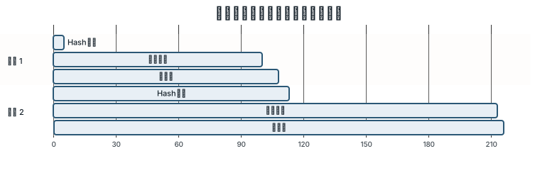
A single 64-bit division takes 80–100 clock cycles! And it can’t be parallelized — each division must complete before the next can begin.

The Smart Trade-off: Powers of Two Instead of Primes

Every textbook says hash table sizes should be prime to reduce collisions. But think carefully: is that cost worth paying?

// Optimized version: use a power of two as the table size
fn is_present_optimized(&self, id: u64) -> bool {
    let mut count = 0;
    let mask = self.table_size - 1;  // table_size must be a power of two

    for i in 0..NUM_HASHES {
        let hash = murmur3_hash(id, i);
        let index = hash & mask;  // bitwise AND replaces modulo!

        if self.bit_array[index] {
            count += 1;
        }
    }

    count == NUM_HASHES
}

Performance comparison:

That’s engineering wisdom: sacrifice a sliver of theoretical perfection (whose real-world impact is negligible) in exchange for a 10x speedup.

The Compiler’s “Magic”: Multiplication Instead of Division

If the divisor is known at compile time, the compiler has another trick up its sleeve:

// Source code
int result = value % 1021;

// Equivalent code generated by the compiler (pseudocode)
uint64_t magic = 0x8102040810204082;  // fixed-point representation of 1/1021
uint64_t temp = value * magic;
int result = value - (temp >> 32) * 1021;

The compiler turned division into multiplication and a shift! This is called “strength reduction.” A 100-cycle division becomes a few-cycle multiply — dozens of times faster.

The Memory Hierarchy: What Really Caps Performance

Branch prediction and execution optimizations are small potatoes. What truly sets the ceiling on performance is memory access.

The Reality of the Cache Hierarchy

What does this hierarchy mean in practice? Take linked-list traversal:

// Linked list node definition
struct Node {
    data: i32,
    next: Option<Box<Node>>,
}

// Approach 1: sequentially allocated linked list (cache-friendly)
// Nodes are laid out contiguously in memory
fn traverse_sequential(head: &Node) -> i32 {
    let mut sum = 0;
    let mut current = Some(head);

    while let Some(node) = current {
        sum += node.data;
        current = node.next.as_deref();
    }
    sum
}

// Approach 2: randomly allocated linked list (cache-hostile)
// Nodes are scattered randomly across memory
fn traverse_random(head: &Node) -> i32 {
    // Identical traversal code, but the nodes live in different places
}

Benchmark results (10 million nodes):

Data Structure	Memory Layout	Traversal Time	Relative Performance
Array	Contiguous	11ms	1.0x
Linked list	Contiguous	24ms	2.2x
Linked list	Random	1300ms	118x

Why such an enormous gap?

1. Array traversal: the CPU prefetcher recognizes the sequential access pattern and pulls data into cache ahead of time.
2. Contiguous linked list: you still have to chase pointers, but since the nodes sit next to each other, cache hit rates stay high.
3. Randomly allocated linked list: nearly every access can miss the cache and must go to main memory — brutally slow.

Pinpointing Bottlenecks with perf

perf’s Top-Down analysis quickly reveals where the problem lies:

# Top-Down performance analysis
perf stat --topdown -a ./program

# Typical output
retiring          : 25.0%  # instructions that retired normally
bad speculation   : 5.0%   # branch mispredictions
frontend bound    : 10.0%  # frontend bottleneck (fetch, decode)
backend bound     : 60.0%  # backend bottleneck (execution, memory)
  - memory bound  : 45.0%  # memory access bottleneck
  - core bound    : 15.0%  # compute resource bottleneck

At a glance the bottleneck is obvious — no more blind guessing and trial-and-error.

The Performance Analysis Toolbox

Knowing the principles is only half the battle; you also need tools that fit your hand.

1. Compiler Explorer: See What the Compiler Is Up To

Compiler Explorer shows the assembly the compiler generates, live:

// Input code
bool has_flag(int value) {
    return value & 0x100;
}

// Output at different optimization levels
// -O0: generates test and a conditional jump
// -O2: generates test and setne (branchless)
// -O3: may be inlined into the call site

2. perf: The Swiss Army Knife of Linux Profiling

# Basic performance counters
perf stat ./program

# Branch prediction analysis
perf stat -e branches,branch-misses ./program

# Cache performance analysis
perf stat -e L1-dcache-loads,L1-dcache-load-misses ./program

# Generate a flame graph
perf record -F 99 ./program
perf script | flamegraph.pl > flamegraph.svg

3. llvm-mca: Static Performance Analysis

# Analyze the performance characteristics of a specific code region
llvm-mca -mcpu=skylake < code.s

# Output includes:
# - instruction throughput
# - port pressure distribution
# - dependency chain analysis
# - resource utilization

Field Notes: Writing Code the CPU Loves

Now that we know all this, what should we watch out for when writing code?

1. Data Organization Beats Algorithmic Tuning

// Bad: AoS (Array of Structures)
struct Particle {
    x: f32, y: f32, z: f32,
    vx: f32, vy: f32, vz: f32,
    mass: f32,
}
let particles: Vec<Particle>;

// Better: SoA (Structure of Arrays)
struct Particles {
    x: Vec<f32>, y: Vec<f32>, z: Vec<f32>,
    vx: Vec<f32>, vy: Vec<f32>, vz: Vec<f32>,
    mass: Vec<f32>,
}

When you’re only updating positions, the SoA layout lets the CPU pull far more useful data per cache line.

2. Reduce Unpredictable Branches

// Bad: unpredictable branch
if random_condition() {
    expensive_operation_a();
} else {
    expensive_operation_b();
}

// Better: compute both up front, decide late
let result_a = compute_a();
let result_b = compute_b();
let result = if condition { result_a } else { result_b };

3. Avoid False Sharing

// Bad: multiple threads touching adjacent data
struct Counters {
    thread1_count: AtomicU64,  // offset 0
    thread2_count: AtomicU64,  // offset 8 — same cache line!
}

// Better: align to cache lines
#[repr(align(64))]  // cache line size
struct Counter {
    value: AtomicU64,
    _padding: [u8; 56],
}

struct Counters {
    thread1_counter: Counter,
    thread2_counter: Counter,
}

4. Lean on the Compiler’s Wisdom

// Give the compiler more information
#[inline(always)]  // force-inline hot functions
#[cold]           // mark a cold path
#[likely]         // branch prediction hint (Rust 1.60+)

// Use const generics to avoid runtime overhead
fn process<const N: usize>(data: &[u8; N]) {
    // The compiler knows N, so it can unroll loops, optimize divisions, etc.
}

Deeper Reflections: Why Must It Be This Complex?

Why Can’t CPUs Just Be Simpler?

You might wonder: why all this complexity — wouldn’t simpler be better? The answer lies in Amdahl’s Law:

Speedup = 1 / ((1 - P) + P/S)

P is the parallelizable fraction and S is the speedup. Even with unlimited cores, the serial portion remains the bottleneck. Single-core performance still matters — which is exactly why CPUs go to such lengths to accelerate serial execution.

RISC vs. CISC: Different Roads, Same Destination

Interestingly, the boundary between RISC and CISC is blurring:

• x86 (CISC): internally decomposes complex instructions into simple micro-ops.
• ARM (RISC): keeps adding complex instructions to improve efficiency.

What does that tell us? In the adult world there is no absolute right or wrong — only trade-offs.

Where Is the Future?

Moore’s Law is running out of steam, and CPU design is exploring new paths:

1. Specialized accelerators: AI chips, dedicated crypto hardware.
2. Near-data computing: move computation next to the data.
3. Quantum computing: rewrite the rules entirely.

But no matter how the technology changes, the fundamentals still matter.

Final Thoughts

A modern CPU is a genuine engineering marvel — billions of transistors coordinating with nanosecond precision. As programmers we don’t need to become hardware experts, but understanding the CPU’s temperament makes our code run faster.

Remember these points:

1. Branch prediction is powerful, but not omnipotent — predictable branches cost almost nothing; random ones are murder.
2. Memory access sets the performance ceiling — algorithmic complexity is theory; cache-friendliness is king.
3. Trust the compiler — give it enough information and it will surprise you.
4. Measure, don’t guess — use the tools.
5. There is no silver bullet — everything is a trade-off.

Next time you hit a performance problem, ask first: does my code match how the CPU actually works? Am I fully exploiting the hardware? Have I stepped on any of these landmines?

Understanding the CPU is like learning a foreign language — hard at first, but once it clicks, a new world opens up. In that world, every clock cycle is precious and every cache hit is worth celebrating.

Remember Knuth’s words: “premature optimization is the root of all evil” — but when optimization is genuinely needed, knowing the principles gives you wings.

May your code always run blazing fast.